Return to computing page for the first course APMA0330
Return to computing page for the second course APMA0340
Return to computing page for the fourth course APMA0360
Return to Mathematica tutorial for the first course APMA0330
Return to Mathematica tutorial for the second course APMA0340
Return to Mathematica tutorial for the fourth course APMA0360
Return to the main page for the course APMA0330
Return to the main page for the course APMA0340
Return to the main page for the course APMA0360
Return to Part I of the course APMA0330
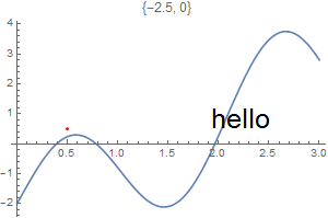
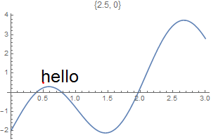
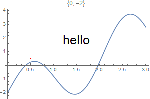
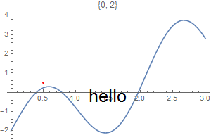
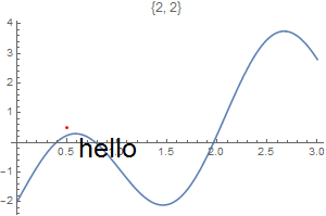
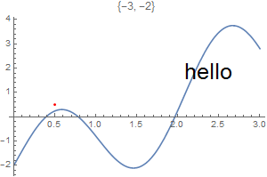
This chapter demonstrates Mathematica capability to generate graphs. We start with its basic command Plot and expose its ability to add text into figures. To place a text inside a figure, Mathematica has a special command Text[expr, coordinates, offset] that specifies an offset for the block of text relative to the coordinate given. Providing an offset < dx, dy >specifies that the point ( x, y ) should lie at relative coordinates < dx, dy >within the bounding rectangle that encloses the text. We demonstrate it with the following codes:
Plot[Sin[x] - Cos[3*x]/3,
The following table of graphs can be displayed using GraphicsGrid command. GraphicsGrid by default puts a narrow border around each of the plots in the array it gives. You can change the size of this border by setting the option Spacings -> < h, v>. The parameters h and v give the horizontal and vertical spacings to be used. The Spacings option uses the width and height of characters in the default font to scale the h and v parameters by default, but it is generally more useful in graphics to use Scaled coordinates. Scaled scales widths and heights so that a value of 1 represents the width and height of one element of the grid.